We assessed racial disparities in policing in the United States by compiling and analysing a dataset detailing nearly 100 million traffic stops conducted across the country. We found that black drivers were less likely to be stopped after sunset, when a ‘veil of darkness’ masks one’s race, suggesting bias in stop decisions. Furthermore, by examining the rate at which stopped drivers were searched and the likelihood that searches turned up contraband, we found evidence that the bar for searching black and Hispanic drivers was lower than that for searching white drivers. Finally, we found that legalization of recreational marijuana reduced the number of searches of white, black and Hispanic drivers—but the bar for searching black and Hispanic drivers was still lower than that for white drivers post-legalization. Our results indicate that police stops and search decisions suffer from persistent racial bias and point to the value of policy interventions to mitigate these disparities.
More than 20 million Americans are stopped each year for traffic violations, making this one of the most common ways in which the public interacts with the police 1,2,3,4 . Due to the decentralized nature of policing in the United States—and a corresponding lack of comprehensive and standardized data—it is difficult to rigorously assess the manner and extent to which race plays a role in traffic stops 5 . The most widely cited national statistics come from the Police–Public Contact Survey (PPCS) 1 , which is based on a nationally representative sample of approximately 50,000 people who report having been recently stopped by the police. In addition to such survey data, some local and state agencies have released periodic reports on traffic stops in their jurisdictions, and have also made their data available to outside researchers for analysis 6,7,8,9,10,11,12,13,14,15,16,17,18,19,20 . While useful, these datasets provide only a partial picture. For example, there is concern that the PPCS, like nearly all surveys, suffers from selection bias and recall errors. Data released directly by police departments are potentially more complete but are available only for select agencies, are typically limited in what is reported and are inconsistent across jurisdictions.
To address these challenges, we compiled and analysed a dataset detailing nearly 100 million traffic stops carried out by 21 state patrol agencies and 35 municipal police departments over almost a decade. This dataset was built through a series of public records requests filed in all 50 states. To facilitate future analysis, we have redistributed these records in a standardized form.
Our statistical analysis of these records proceeds in three steps. First, we assess potential bias in stop decisions by applying the ‘veil of darkness’ test developed by Grogger and Ridgeway 21 . This test is based on a simple observation: because the sun sets at different times throughout the year, one can examine the racial composition of stopped drivers as a function of sunlight while controlling for time of day. In particular, we use the discontinuity created by the start (and end) of daylight-saving time (DST), comparing the racial distribution of drivers stopped in the evenings immediately before DST begins, when it is dark, to the distribution after DST begins, when it is light at the same time of day. If black drivers comprise a smaller share of stopped drivers when it is dark and accordingly difficult to determine a driver’s race, that suggests black drivers were stopped during daylight hours in part because of their race. In both state patrol and municipal police stops, we find that black drivers comprise a smaller proportion of drivers stopped after sunset, suggestive of discrimination in stop decisions.
Second, we investigate potential bias in the post-stop decision to search drivers for contraband. To do so, we apply the threshold test recently developed by Simoiu et al. 7 and refined by Pierson et al. 22 . The threshold test incorporates both the rate at which searches occur, as well as the success rate of those searches, to infer the standard of evidence applied when determining whom to search. This approach builds on traditional outcome analysis 23,24 , in which a lower search success rate for one group relative to another is seen as evidence of bias against that group, as it suggests that a lower evidentiary bar was applied when making search decisions. Applied to our data, the threshold test indicates that black and Hispanic drivers were searched on the basis of less evidence than white drivers, both on the subset of searches carried out by state patrol agencies and on those carried out by municipal police departments.
Finally, we examine the effects of drug policy on racial disparities in traffic stop outcomes. We specifically compare patterns of policing in Colorado and Washington—two states that legalized recreational marijuana at the end of 2012—to those in 12 states in which recreational marijuana remained illegal. Using a difference-in-differences strategy, we find that legalization reduced both search rates and misdemeanour rates for drug offences for white, black and Hispanic drivers—though a gap in search thresholds persists.
In the process of collecting and analysing millions of traffic stop records across the country, we encountered many logistical and statistical challenges. Based on these experiences, we conclude by offering suggestions to improve data collection, analysis and reporting by law enforcement agencies. Looking forward, we hope this work provides a road map for measuring racial disparities in policing, and facilitates future empirical research into police practices.
To assemble a national dataset of traffic stops, we filed public records requests with all 50 state patrol agencies and over 100 municipal police departments. The municipal police departments include those that serve the largest 100 cities in the nation; to achieve geographic coverage, we also included departments that serve some of the largest cities in each state.
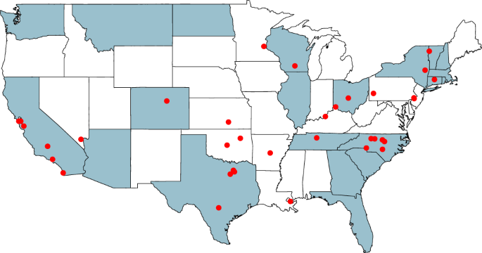
To date, we have collected (and released) data on approximately 221 million stops carried out by 33 state patrol agencies, and 34 million stops carried out by 56 municipal police departments, for a total of 255 million records. In many cases, however, the data we received were insufficient to assess racial disparities (for example, the race of the stopped driver was not regularly recorded, or only a non-representative subset of stops was provided). For consistency in our analysis, we further restrict to stops occurring in 2011–2018, as many jurisdictions did not provide data on earlier stops. Finally, we limit our analysis to drivers classified as white, black or Hispanic, as there were relatively few recorded stops of drivers in other race groups. Our primary dataset thus consists of approximately 95 million stops from 21 state patrol agencies and 35 municipal police departments, as shown in Fig. 1 and described in more detail in Supplementary Table 2.
Because each jurisdiction provided stop data in idiosyncratic formats with varying levels of specificity, we used a variety of automated and manual procedures to create the final dataset. For each recorded stop, we attempted to extract and normalize the date and time of the stop; the county (for state patrol agencies) or police subdivision (for example, beat, precinct or zone, for municipal police departments) in which the stop took place; the race, gender and age of the driver; the stop reason (for example, speeding); whether a search was conducted; the legal justification for the search (for example, ‘probable cause’ or ‘consent’); whether contraband was found during a search; and the stop outcome (for example, a citation or an arrest). As indicated in Supplementary Table 2, the information we received varies markedly across states. We therefore restricted each of our specific analyses to the corresponding subset of jurisdictions for which we have the required fields. Our complete data-cleaning pipeline is extensive and required subjective decisions, which we describe in more detail in Methods. For transparency and reproducibility, we have released the raw data, the standardized data and code to clean and analyse the records at https://openpolicing.stanford.edu.
Relative to their share of the residential population, we found that black drivers were, on average, stopped more often than white drivers. In particular, among state patrol stops, the annual per-capita stop rate for black drivers was 0.10 compared to 0.07 for white drivers; and among municipal police stops, the annual per-capita stop rate for black drivers was 0.20 compared to 0.14 for white drivers. For Hispanic drivers, however, we found that stop rates were lower than for white drivers: 0.05 for stops conducted by state patrol (compared to 0.07 for white drivers) and 0.09 for those conducted by municipal police departments (compared to 0.14 for white drivers). In all cases, these numbers are the unweighted average annual per-capita stop rates across the states and cities we analysed, and all estimates have corresponding 95% confidence intervals (CIs) with radius
These numbers are a starting point for understanding racial disparities in traffic stops, but they do not, per se, provide strong evidence of racially disparate treatment. In particular, per-capita stop rates do not account for possible race-specific differences in driving behaviour, including amount of time spent on the road and adherence to traffic laws. For example, if black drivers, hypothetically, spend more time on the road than white drivers, that could explain the higher stop rates we see for the former, even in the absence of discrimination. Moreover, drivers may not live in the jurisdictions where they were stopped, further complicating the interpretation of population benchmarks.
Quantifying potential bias in stop decisions is a statistically challenging problem, in large part because one cannot readily measure the racial distribution of those who actually violated traffic laws because the data contain information only on those stopped for such offences. To mitigate this benchmarking problem, Grogger and Ridgeway 21 proposed a statistical approach known as the veil-of-darkness test. Their method starts from the idea that officers who engage in racial profiling are less able to identify a driver’s race after dark than during the day. As a result, if officers are discriminating against black drivers—all else being equal—one would expect black drivers to comprise a smaller share of stopped drivers at night, when a veil-of-darkness masks their race. To account for patterns of driving and police deployment that may vary throughout the day, the test leverages the fact that the sun sets at different times during the year. For example, although it is typically dark at 19:00 during the winter months, it is often light at that time during the summer.
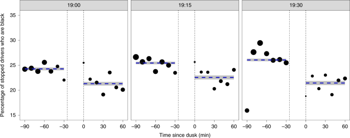
To illustrate the intuition behind this method, in Fig. 2 we examine the demographic composition of drivers stopped by the Texas State Patrol at various times of day. Each panel in the plot shows stops occurring in a specific 15-min window (for example, 19:00–19:15), and the horizontal axis indicates minutes since dusk. We restrict to white and black drivers—because the ethnicity of Hispanic drivers is not always apparent, even during daylight hours—and, following Grogger and Ridgeway, we filter out stops that occurred in the ~30-min period between sunset and dusk, when it is neither ‘light’ nor ‘dark.’ For each time period, the plot shows a marked drop in the proportion of drivers stopped after dusk who are black, suggestive of discrimination in stop decisions.
In this basic form, darkness—after adjusting for time of day—is a function of the date. As such, to the extent that driver behaviour changes throughout the year, and that these changes are correlated with race, the test can suggest discrimination where there is none. To account for these potential seasonal effects, we applied a more robust variant of the veil-of-darkness test that restricts to two 60-day windows centred on the beginning and end of DST 25 . On this subset of the data, we fit the following logistic regression model:
where Pr(black ∣ t, g, p, d, s, c) is the probability that a stopped driver is black at a certain time t, location g and period p (with two periods per year, corresponding to the start and end of DST), with darkness status d ∈ indicating whether a stop occurred after dusk (d = 1) or before sunset (d = 0), and with the enforcement agency being either state patrol, s ∈ or city police department, c ∈ . In this model, ns6(t) is a natural spline over time with six degrees of freedom, γ[g] is a fixed effect for location g and δ[p] is a fixed effect for period p. The location g[i] for stop i corresponds to either the county (for state patrol stops) or city (for municipal police department stops), with γ[g[i]] the corresponding coefficient. Finally, p[i] captures whether stop i occurred in the spring (within a month of beginning DST) or the fall (within a month of ending DST) of each year, and δ[p[i]] is the corresponding coefficient for this period. For computational efficiency, we rounded time to the nearest 5-min interval when fitting the model.
The veil-of-darkness test is a popular technique for assessing disparate treatment but, like all statistical methods, it comes with caveats. Results could be skewed if race-specific driving behaviour is related more to lighting than time of day, leading the test to suggest discrimination where there is none. Conversely, artificial lighting (for example, from street lamps) can weaken the relationship between sunlight and visibility, and so the method may underestimate the extent to which stops are predicated on perceived race. Finally, if violation type is related to lighting, the test could give an inaccurate measure of discrimination. For example, broken tail lights are more likely to be detected at night and could potentially be more common among black drivers 17 , which could in turn mask discrimination. To address this last limitation, one could exclude stops prompted by such violations but our data, unfortunately, do not consistently indicate stop reasons. Despite these shortcomings, we believe the veil-of-darkness test provides a useful, if imperfect, measure of bias in stop decisions.
After stopping a driver, officers may carry out a search of the driver or vehicle if they suspect more serious criminal activity. We next investigate potential bias in these search decisions. Among stopped drivers, we found that black and Hispanic individuals were, on average, searched more often than white individuals. However, as with differences in stop rates, the disparities we see in search rates are not necessarily the product of discrimination. Black and Hispanic drivers might, hypothetically, carry contraband at higher rates than white drivers, and so elevated search rates may result from routine police work even if no racial bias were present. To measure the role of race in search decisions, we apply two statistical strategies: outcome analysis and threshold analysis. To do so, we limit to the eight state patrol agencies and six municipal police departments for which we have sufficient data on the location of stops, whether a search occurred and whether those searches yielded contraband. We specifically consider state patrol agencies in Connecticut, Illinois, North Carolina, Rhode Island, South Carolina, Texas, Washington and Wisconsin; and municipal police departments in Nashville, TN, New Orleans, LA, Philadelphia, PA, Plano, TX, San Diego, CA and San Francisco, CA. We defer to each department’s characterization of ‘contraband’ when carrying out this analysis.
In these jurisdictions, stopped black and Hispanic drivers were searched about twice as often as stopped white drivers. To assess whether this gap resulted from biased decision-making, we apply the outcome test, originally proposed by Becker 23,24 , to circumvent omitted variable bias in traditional tests of discrimination. The outcome test is based not on the search rate but on the ‘hit rate’: the proportion of searches that successfully turn up contraband. Becker argued that even if minority drivers are more likely to carry contraband, in the absence of discrimination, searched minorities should still be found to have contraband at the same rate as searched whites. If searches of minorities are successful less often than searches of whites, it suggests that officers are applying a double standard, searching minorities on the basis of less evidence. Implicit in this test is the assumption that officers exercise discretion in whom to search; therefore, when possible, we exclude non-discretionary searches, such as vehicle impound searches and searches incident to arrest, as those are often required as a matter of procedure, even in the absence of individualized suspicion. We note that outcome tests gauge discrimination only at one specific point in the decision-making process—in this case, the decision to search a driver who has been stopped. In particular, this type of analysis does not capture bias in the stop decision itself.
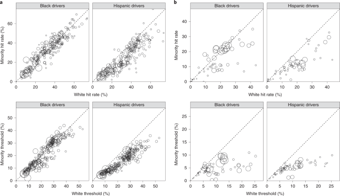
In Fig. 3 (top row), we plot hit rates by race and location for the states (left) and for the cities (right) for which we have the necessary information. Across jurisdictions, we consistently found that searches of Hispanic drivers were less successful than those of white drivers. However, searches of white and black drivers had more comparable hit rates. The outcome test thus indicates that search decisions may be biased against Hispanic drivers, but the evidence is more ambiguous for black drivers. Aggregating across state patrol stops, contraband was found in 32.0% (95% CI 31.6–32.4%) of searches of white drivers compared to 24.3% (95% CI 23.5–25.2%) of searches of Hispanic drivers and 29.4% (95% CI 28.7–30.0%) of searches of black drivers. In particular, the gap in hit rates between white and Hispanic drivers was 7.6% (95% CI 6.7–8.6%, P < 0.001), and the gap in hit rates between white and black drivers was 2.6% (95% CI 1.9–3.4%, P < 0.001). Similarly, aggregating across municipal police departments, contraband was found in 18.2% (95% CI 17.8–18.7%) of searches of white drivers compared to 11.0% (95% CI 10.6–11.5%) of searches of Hispanic drivers and 13.9% (95% CI 13.7–14.2%) of searches of black drivers. In this case, the gap in hit rates between white and Hispanic drivers was 7.2% (95% CI 6.6–7.8%, P < 0.001) and the gap in hit rates between white and black drivers was 4.3% (95% CI 3.8–4.8%, P < 0.001). These numbers all indicate unweighted averages across our cities and states, respectively.
The outcome test is intuitively appealing, but it is an imperfect barometer of bias; in particular, it suffers from the problem of infra-marginality 8,26,27 . To illustrate this shortcoming, suppose that there are two, easily distinguishable, types of white driver: those who have a 5% chance of carrying contraband and those who have a 75% chance of carrying contraband. Likewise assume that black drivers have either a 5 or 50% chance of carrying contraband. If officers search drivers who are at least 10% likely to be carrying contraband, then searches of white drivers will be successful 75% of the time whereas searches of black drivers will be successful only 50% of the time. Thus, although the search criterion is applied in a race-neutral manner, the hit rate for black drivers is lower than that for white drivers and the outcome test would (incorrectly) conclude that searches are biased against black drivers. The outcome test can similarly fail to detect discrimination when it is present.
Addressing this possibility, Knowles et al. 27 suggested an economic model of behaviour—known as the KPT model—in which drivers balance their utility for carrying contraband with the risk of getting caught, while officers balance their utility of finding contraband with the cost of searching. Under equilibrium behaviour in this model, the hit rate of searches is identical to the search threshold and so one can reliably detect discrimination with the standard outcome test. However, Engel and Tillyer 28 argue that the KPT model of behaviour requires strong assumptions, including that drivers and officers are rational actors and that every driver has perfect knowledge of the likelihood that he or she will be searched.
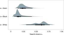
To mitigate the limitations of outcome tests (as well as limitations of the KPT model), the threshold test has been proposed as a more robust means for detecting discrimination 7,22 . This test aims to estimate race-specific probability thresholds above which officers search drivers—for example, the 10% threshold in the hypothetical situation above. Even if two race groups have the same observed hit rate, the threshold test may find that one group is searched on the basis of less evidence, indicative of discrimination. To accomplish this task, the test uses a Bayesian model to simultaneously estimate race-specific search thresholds and risk distributions that are consistent with the observed search and hit rates across all jurisdictions. The threshold test can thus be seen as a hybrid between outcome and benchmark analysis, as detailed in Methods.
As shown in Fig. 3 (bottom row), the threshold test indicates that the bar for searching black and Hispanic drivers is generally lower than that for searching white drivers across the municipal police departments and states we consider. In aggregate across cities, the inferred threshold for white drivers is 10.0% compared to 5.0 and 4.6% for black and Hispanic drivers, respectively. The estimated gaps in search thresholds between white and non-white drivers are large and statistically significant: the 95% credible interval for the Hispanic–white difference is (–6.4, –4.4%) and the corresponding interval for the black–white difference is (–6.1, –4.0%). Similarly across states, the inferred threshold for white drivers is 20.9% compared to 16.0% for black drivers and 13.9% for Hispanic drivers. These differences are again large and statistically significant: the 95% credible interval for the Hispanic–white gap is (–8.4, –5.6%); and the analogous interval for the black–white gap is (–6.5%, –3.1%). As with our outcome results, aggregate thresholds are computed by taking an unweighted average of the city- and state-specific thresholds, respectively.
Compared to by-location hit rates, the threshold test more strongly suggests discrimination against black drivers, particularly for municipal stops. Consistent with past work 7 , this difference appears to be driven by a small but disproportionate number of black drivers who have a high inferred likelihood of carrying contraband. Thus, even though the threshold test finds that the bar for searching black drivers is lower than that for white drivers, these groups have more similar hit rates.
The threshold test provides evidence of racial bias in search decisions. However, as with all tests of discrimination, it is important to acknowledge limits in what one can conclude from such statistical analysis per se. For example, if search policies differ not only across, but also within, the geographic subdivisions we consider, then the threshold test might mistakenly indicate discrimination where there is none. Additionally, if officers disproportionately suspect more serious criminal activity when searching black and Hispanic drivers compared to white drivers (for example, possession of larger quantities of contraband), then lower observed thresholds may stem from non-discriminatory police practices. Finally, we note that thresholds cannot be identified by the observed data alone 7 , and so inferences are dependent on the specific functional form of the underlying Bayesian model, including the prior distributions. (In Methods, however, we show that our main results are robust to relatively large changes to prior distributions).
We conclude our analysis by investigating the effects of legalization of recreational marijuana on racial disparities in stop outcomes. We specifically examine Colorado and Washington, two states in which marijuana was recently legalized and for which we have detailed data before and after legalization. In line with expectations, we find that the proportion of stops that resulted in either a drug-related infraction or misdemeanour fell substantially in both states after marijuana was legalized at the end of 2012 (see Supplementary Fig. 2). Notably, since black drivers were more likely to be charged with such offences previous to legalization, these drivers were also disproportionately impacted by the policy change. This finding is consistent with past work showing that marijuana laws disproportionately affect minorities 29 .
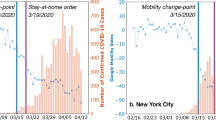
Because the policy change decriminalized an entire class of behaviour (that is, possession of small amounts of marijuana), it is not surprising that drug offences correspondingly decreased. However, it is less clear, a priori, how the change might have affected officer behaviour more broadly. Investigating this issue, we found that after the legalization of marijuana the number of searches fell substantially in Colorado and Washington (Fig. 4), ostensibly because the policy change removed a common reason for conducting searches.
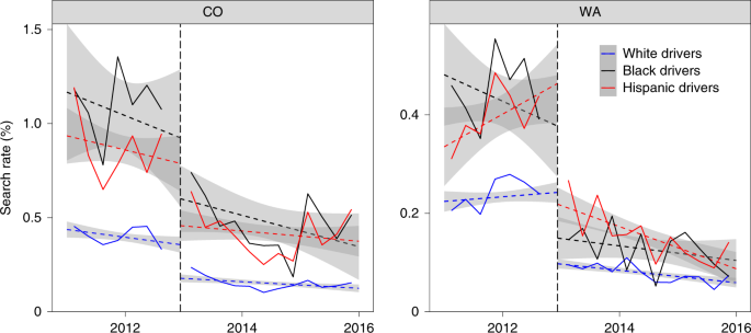
Because black and Hispanic drivers were more likely to be searched before legalization, the policy change reduced the absolute gap in search rates between race groups; however, the relative gap persisted, with black and Hispanic drivers still more likely to be searched than white drivers post-legalization. We further note that marijuana legalization had secondary impacts for law-abiding drivers, because fewer searches overall also meant fewer searches of those without contraband. In the year after legalization in Colorado and Washington, about one-third fewer drivers were searched with no contraband found than in the year before legalization.
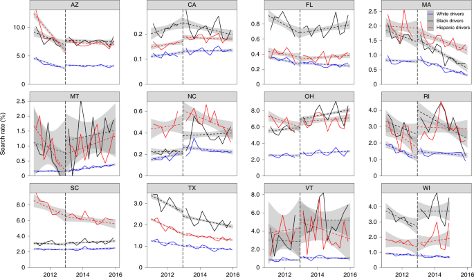
As further evidence that the observed drop in search rates in Colorado and Washington was due to marijuana legalization, we note that in the 12 states where marijuana was not legalized—and for which we have the necessary data—search rates did not exhibit sharp drops at the end of 2012 (Fig. 5). To add quantitative detail, we computed a difference-in-differences estimate 30 ; our precise model specification and the fitted coefficients are described in Methods. We found that the race-specific coefficients are large and negative for white, black and Hispanic drivers, which again suggests that the observed drop in searches in Colorado and Washington was caused by the legalization of marijuana in those states.
Despite the legalization of marijuana decreasing search rates across race groups, Fig. 4 shows that the relative disparity between whites and minorities remained. We applied the threshold test to assess the extent to which this disparity in search rates may reflect bias. Examining the inferred thresholds (shown in Supplementary Fig. 3), we found that white drivers faced consistently higher search thresholds than minority drivers, both before and after marijuana legalization. The data thus suggest that, although overall search rates dropped in Washington and Colorado, black and Hispanic drivers still faced discrimination in search decisions.
Analysing nearly 100 million traffic stops across the country, we have worked to quantify the often complex relationship between race and policing in the United States. Our analysis provides evidence that decisions about whom to stop and, subsequently, whom to search are biased against black and Hispanic drivers. Our results, however, also point to the power of policy interventions—specifically, legalization of recreational marijuana—to reduce these racial disparities.
These findings lend insight into patterns of policing, but they only partially capture the wider impacts of law enforcement on communities of colour. If, for example, officers disproportionately patrol black and Hispanic neighbourhoods, the downstream effects can be injurious even if individual stop decisions are not directly affected by the colour of one’s skin. Similarly, enforcement of minor traffic violations, like broken tail lights—even if conducted uniformly and without animus—can place heavy burdens on black and Hispanic drivers without improving public safety 17 . We hope the data we have collected and released are useful for measuring, and in turn addressing, these broader effects.
In the course of carrying out this study, we encountered many challenges working with large-scale policing data. We conclude by offering several recommendations for future data collection, release and analysis. As a minimum, we encourage jurisdictions to collect individual-level stop data that include the date and time of the stop; the location of the stop; the race, gender and age of the driver; the stop reason; whether a search was conducted; the search type (for example, ‘probable cause’ or ‘consent’); whether contraband was found during a search; the stop outcome (for example, a citation or an arrest); and the specific violation with which the driver was charged. Most jurisdictions collect only a subset of this information. There are also variables that are currently rarely collected but would be useful for analysis, such as indicia of criminal behaviour, an officer’s rationale for conducting a search and short narratives written by officers describing the incident. New York City’s UF-250 form for pedestrian stops is an example of how such information can be efficiently collected 31,32 .
Equally important to data collection is ensuring the integrity of the recorded information. We frequently encountered missing values and errors in the data (for example, implausible values for a driver’s age and invalid racial categorizations). Automated procedures can be put in place to help detect and correct such problems. For example, the recorded race of the driver is often based on the officer’s perception rather than a driver’s self-categorization. While there are perhaps sound reasons for this practice, it increases the likelihood of errors. To quantify and correct for this issue, police departments might regularly audit their data, possibly by comparing an officer’s perception of race to a third party’s judgement based on driver’s licence photos for a random sample of stopped drivers.
Despite the existence of public records laws, several jurisdictions failed to respond to our repeated requests for information. We hope that law enforcement agencies consider taking steps to make data more accessible to both external researchers and the public. Connecticut and North Carolina are at the forefront of opening up their data, providing online portals for anyone to download and analyse this information.
We also hope that police departments start to analyse their data regularly and report the results of their findings. Such analyses might include estimates of stop, search and hit rates stratified by race, age, gender and location; distribution of stop reasons by race; and trends over time. More ambitiously, departments could use their data to design statistically informed guidelines that encourage more consistent, efficient and equitable decisions 31,33,34,35 . Many of these analyses can be automated and rerun regularly with little marginal effort. In conjunction with releasing the data underlying these analyses, we recommend that the analysis code also be released to ensure reproducibility.
Finally, it bears emphasis that the type of large-scale data analysis we have carried out in this paper is but one of many complementary ways to gauge and rectify bias in police interactions with the public. Just as critical, for example, are conversations with both officers and community members, who can often provide more nuance than is possible with our aggregate statistical approach. Collecting, releasing and analysing police data are important steps for increasing the effectiveness and equity of law enforcement practices, and for improving relations with the public through transparency. Ultimately, though, data collection and analysis are not enough. We must act on the results of such efforts if we are to reduce the persistent, discriminatory impacts of policing on communities of colour.
Our primary dataset includes 94,778,505 stops from 21 state patrol agencies and 35 municipal police departments. For more detail on all jurisdictions whose data were used in our analyses, Supplementary Table 2 lists the total number of stops and the range of years in which these stops took place. The table also indicates whether each of several important covariates was available in each jurisdiction: the date and time of the stop; more granular geographic information; the race, age and gender of the stopped driver; and whether a search was conducted and, if so, whether contraband was found. Our data-processing pipeline was extensive. Below we describe some of the key steps in this process, and also note that the complete code required to process the data is available at https://openpolicing.stanford.edu.
For each state and city, we requested individual-level records for traffic stops conducted since 2005, under the state’s public records law and filed with the agency responsible for traffic stop data collection. The 33 states and 56 cities that complied provided the data in various formats, including raw text files, Microsoft Excel spreadsheets and Microsoft Access databases. We converted all data we received to a standard comma-separated, text-file format. The states and cities varied widely in terms of the availability of the different data fields, the manner and detail of how the data were recorded and in recording consistency from year to year, even within the same location.
We standardized available fields when possible. Often, locations provided dictionaries to map numeric values to human-interpretable ones. Aggregated data—as provided by Missouri, Nebraska and Virginia, for example—were disaggregated by expanding the number of rows by the reported count. For some locations, we had to manually map the provided location data to a county or district value. For example, in Washington, counties were mapped by first computing the latitude and longitude of the highway post that was recorded for the stop, and then those coordinates were mapped to a county using a shapefile. The raw data we received from the states and cities, the processed data we used in this analysis and the code to clean and analyse the data are all available for public inspection and reuse.
In many cases, more than one row in the raw data appeared to refer to the same stop. For example, in several jurisdictions each row in the raw data referred to one violation, not one stop. We detected and reconciled such duplicates by matching on a location-specific set of columns. For example, in Colorado we counted two rows as duplicates if they had the same officer identification code, officer first and last name, driver first and last name, driver birth date, stop location (precise to the milepost marker) and stop date and time. This type of de-duplication was a common procedure that we applied to many states and cities.
The raw data provided to us by state and municipal police agencies often contained clear errors. We ran numerous automated checks to detect and correct these where possible, although some errors probably remain due to the complex nature of the data. For example, after examining the distribution of recorded values in each jurisdiction, we discovered a spurious density of stops in North Carolina listed as occurring at precisely midnight. As the value ‘00:00’ was probably used to indicate missing information, we treated it as such. In Pittsburgh, PA, recorded values for ‘sex’ and ‘gender’ did not match 73% of the time in the pedestrian stop data, suggesting data corruption. (Note that we did not include pedestrian stop data in our analysis, but we have released those records for other researchers to use.)
In another example, past work revealed that Texas State Patrol officers incorrectly recorded many Hispanic drivers as white, an error the agency subsequently corrected 36 . To investigate and adjust for this issue, we imputed Hispanic ethnicity from surnames. To carry out this imputation, we used a dataset from the U.S. Census Bureau that estimates the racial and ethnic distribution of people with a given surname for surnames occurring at least 100 times 37 . To increase the matching rate, we performed minor string edits to the names, including removal of punctuation and suffixes (for example, ‘Jr.’ and ‘II’), and considered only the longest word in multi-part surnames. Following previous studies 38,39 , we defined a name as ‘typically’ Hispanic if at least 75% of people with that name identified as Hispanic, and we note that 90% of those with typically Hispanic names identified as Hispanic in the 2000 Census.
Among drivers with typically Hispanic names, the proportion labelled as Hispanic in the raw data was quite low in Texas (37%), corroborating past results. For comparison, we considered Arizona and Colorado, the two other states that included driver name in the raw data. The proportion of drivers with typically Hispanic names labelled as Hispanic in the raw data was 70% in Colorado and 79% in Arizona, much higher than in Texas. Because of this known issue in the Texas data, we re-categorized as ‘Hispanic’ all drivers in Texas with Hispanic names who were originally labelled ‘white’ or who had missing race data; this method adds about 1.9 million stops of Hispanic drivers over the period 2011–2015. We did not re-categorize drivers in any other jurisdiction.
In our veil-of-darkness analysis, we compared stop rates before sunset and after dusk—as is common when applying this test. Specifically, sunset is defined as the point in time where the sun dips below the horizon, and dusk (also known as the end of civil twilight) is the time when the sun is six degrees below the horizon and when it is generally considered to be ‘dark.’ As recommended by Grogger and Ridgeway 21 , we further restricted to stops that occurred during the ‘inter-twilight period’: the range from the earliest to the latest time that dusk occurs in the year. This range is approximately 17:00–22:00, although the precise values differ by location and year. All times in the inter-twilight period are, by definition, light at least once in the year and dark at least once in the year. In Supplementary Table 1, we report the results of several variations of our primary veil-of-darkness model (for example, varying the degree of the natural spline from 1 to 6). The results were statistically significant and qualitatively similar in all cases.
The threshold test for discrimination was introduced by Simoiu et al. 7 to mitigate the most serious shortcomings of benchmark and outcome analysis. The test is informed by a stylized model of officer behaviour. During each stop, officers observe a myriad of contextual factors—including the age, gender and race of the driver, and behavioural indicators of nervousness or evasiveness. We imagine that officers distil all these complex signals down to a single number, p, that represents their subjective estimate of the likelihood that the driver is carrying contraband. Based on these factors, officers are assumed to conduct a search if, and only if, their subjective estimate of finding contraband, p, exceeds a fixed, race-specific search threshold for each location (for example, county or district). Treating both the subjective probabilities and the search thresholds as latent, unobserved quantities, our goal is to infer them from data. The threshold test takes a Bayesian approach to estimating the parameters of this process, with the primary goal of inferring race-specific search thresholds for each location.
Under this model of officer behaviour, we interpret lower search thresholds for one group relative to another as evidence of discrimination. If, for example, officers have a lower threshold for searching black drivers than white drivers, that would indicate that they are willing to search black drivers on the basis of less evidence than for white drivers—and we would conclude that black drivers are being discriminated against. In the economics literature, this type of behaviour is often called taste-based discrimination 24 as opposed to statistical discrimination 40,41 , in which officers might use a driver’s race to improve their estimate that the driver is carrying contraband. Regardless of whether such information increases the efficiency of searches, officers are legally barred from using race to inform search decisions outside of circumscribed situations (for example, when acting on specific and reliable suspect descriptions that include race among other factors). The threshold test, however, aims to capture only taste-based discrimination, as is common in the empirical literature on discrimination.
In our work, we applied a computationally fast variant of the threshold test developed by Pierson et al. 22 , which we fit separately on both state patrol stops and municipal police stops. As described below, we modified the Pierson et al. test to include an additional hierarchical component. For example, while the original Pierson et al. model considered one state, and allowed parameters to vary by county (and race) within that state, our state patrol model considers multiple states, allowing parameters to vary by county (and race) within each state. Relevant information is partially pooled across both counties and states. Similarly, our municipal model considers multiple police departments, allowing parameters to vary by police district (and race) within each department.
To run the threshold test, we assume the following information is observed for each stop, i:
To formally describe the threshold test, we need to specify the parametric process of search and recovery, as well as the priors on those parameters. For ease of exposition, we present the model for state patrol stops, where stops occur in counties that are nested within states. The municipal stop model has the same structure, with districts corresponding to counties and cities corresponding to states. We start by describing the latent signal distributions on which officers base their search decisions, which we parameterize by the race and location of drivers. As detailed in Pierson et al. 22 , these signal distributions are modelled as homoskedastic discriminant distributions, a class of logit-normal mixture distributions supported on the unit interval [0, 1]. Discriminant distributions can closely approximate beta distributions, but they have properties that are computationally attractive. Each race- and county-specific signal distribution can be described using two parameters, which we denote by ϕr,d and δr,d. In our setting, ϕr,d ∈ (0, 1) is the proportion of drivers of race r in county d that carry contraband; and δr,d > 0 characterizes how difficult it is to identify drivers with contraband 34 .
We impose additional structure on the signal distributions by assuming that ϕr,d and δr,d can be decomposed into additive race and location terms. Specifically, given parameters ϕr,g for each race group r and state g, and parameters ϕd for each county d, we set
where g[d] denotes the state g in which county d lies. Similarly, for parameters δr,g and δd, we set
Following Pierson et al. 22 , we use hierarchical priors 42 on the signal distributions that restrict geographical heterogeneity while allowing for base rates to differ across race groups. This choice substantially accelerates model fitting. In particular, we use the following priors: